5 Discussion
This chapter discusses in greater depth the results presented in the previous chapter, explaining these results and their implications.
Broadly, the discussion focuses on the two key concerns of the dissertation: the creation of spatial segmentations which reflect the urban morphology of a city, and the creation of spatial segmentations which can be used as spatial housing submarkets. Certain measures and evaluations of the segmentations focus on one or the other of these concerns—for instance the QCoD assesses solely the segmentations’ suitability to represent housing submarkets—while other assessments of the segmentation are germane to both concerns. Many of the key findings are of a methodological nature, demonstrating the ways in which altering certain elements of the methodology affects the segmentation produced. These methodological findings often correspond to limitations in the research, and more broadly in the methodology employed.
5.1 Creating spatial segmentations to reflect housing submarkets
As reported in the previous chapter, the QCoD allows the degree to which segmentations capture variation in house prices to be quantified, allowing comparisons between different segmentations to be made on this criterion.
The similar type-level average QCoD values for the MT, ET, ET transposed to H3, and ET transposed to block segmentations (see Figure 4.10) suggest that transposing to the H3 or block geometry has minimal effect on the degree of house price variation captured by the segmentation. This kind of transposition may therefore be a good way to reduce the ‘fragmentary’ nature of the segmentation and ‘clean up’ its geometry to a certain extent, without damaging its performance with regards to delineating housing submarkets.
Figure 4.10 also highlights the difficulties of making direct comparisons between segmentations which divide an area into a different number of units and/or units with different areas. The existing neighbourhoods and idealista polygons have lower QCoDs than any of the novel segmentations, but they also have significantly lower average type areas and a higher number of types, and so to some extent this should be expected. Interestingly, judging solely on the metrics shown in Figure 4.10 could lead to the conclusion that the spatially constrained segmentation performs very well; however the geographical distribution of its clusters (see Figure 4.7) means that the segmentation would likely be of little use in practice.
A comparison of Figure 4.10 and Figure 4.12 highlights the different conclusions reached when different spatial units (the type and polygon) are used as the basis for analysis. While the positions of segmentations on each chart varies, certain key trends are true of both. Both demonstrate the general relationship between average unit area and average unit QCoD, and in both most of the novel segmentations form a cluster of relatively similar values, suggesting relatively small differences between the performances of these segmentations on the metrics plotted on these charts10.
5.2 Creating coherent spatial segmentations
5.2.1 Fragmentary segmentations
Throughout the process of producing spatial segmentations, one issue encountered was that the spatial units generated were fragmentary and had limited spatial contiguity. When using the GMM algorithm to cluster base spatial units, the clustering algorithm has no knowledge of the topological relationships between the cells it is clustering, and as such there is no guarantee that any segmentations produced will be contiguous. The fragmentary kinds of segmentations produced by such clusterings cannot be seen to accurately represent either urban morphology or housing submarkets: although the specific details may differ dependent on the conceptualisation and scale of either of these areas, both are certainly larger than the tessellation cells used in ET/MT-based segmentations. Hence, a segmentation which assigns an individual ET/MT cell different cluster labels to all of its neighbours can be seen to have failed to adequately delineate either urban tissues or housing submarkets: in this resultant segmentation, the single tessellation cell will be classed as a distinct polygon, but will not by any reasonable measure be representative of the concepts it seeks to represent.
An argument could be made that, while using the ‘polygons’ of the segmentation makes more conceptual sense when using the segmentations to represent housing submarkets, different types of urban morphology may be better conceptually aligned with the ‘types’ of the segmentation, and therefore fragmentary segmentations are less problematic when classifying urban morphology.
5.2.2 Limiting fragmentary segmentations with contextual characters
As explained in the Methodology, an imperfect solution to the problem of fragmented segmentations is the use of contextual characters constructed by averaging the values of nearby cells. Indeed, these are incorporated into all segmentations presented in the previous chapter (save that which stipulated a spatial constraint). Figure 5.1 demonstrates the difference that changing the neighbour criteria when generating contextual characters makes to the final segmentation. While vague spatial patterns can be discerned, the clustering using only the primary characters of each cell (on the far left) is far too fragmented to offer a useful segmentation of either urban morphology or housing submarkets. The subsequent maps plot segmentations identical in all factors save the neighbour criteria used to generate the contextual characters, showing clusterings based on contextual characters built using neighbours up to a topological distance of one, three, and five.
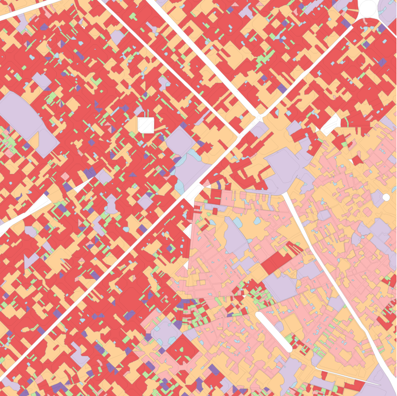
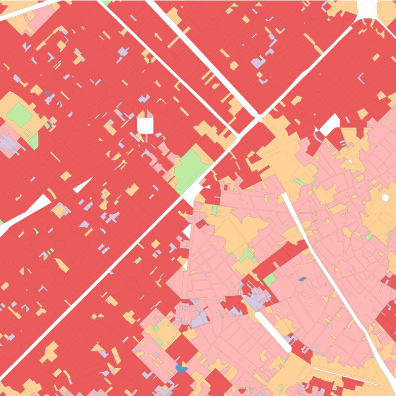
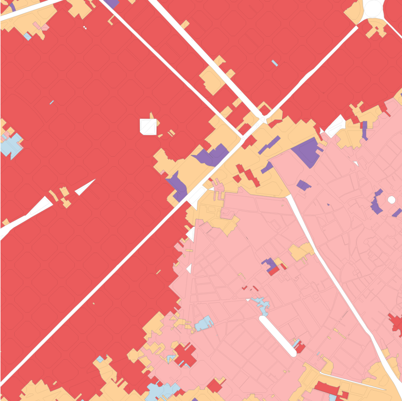
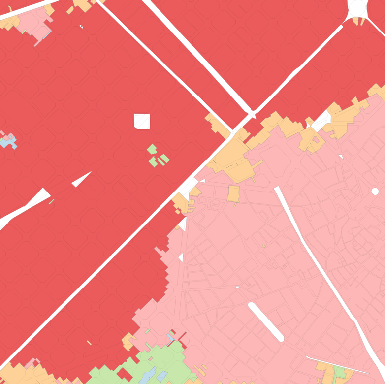
Figure 5.1: The effect of an otherwise identical segmentation on contextual characters constructed using different order spatial weights. From left to right: no contextual characters; 1st order spatial weight, up to 3rd order spatial weight, up to 5th order spatial weight.
Besides acting simply as a methodological tool to create cleaner segmentations, contextual characters also serve a conceptual role. The central reason that the segmentation using only primary characters is too fragmented to be of any practical use is that the tessellation cells clustered (aspatially, with GMM) hold no information about their ‘surroundings’. The urban morphology of a given tissue cannot, however, be defined based only on one building (or tessellation cell). Accordingly, the contextual characters serve to partially determine the scale of the areas demarcated in the resultant segmentation: the wider the range of neighbours included in the contextual characters, the larger (in general) the polygons in the resultant segmentation will be.
The choice of topological distance used to determine the contextual characters should therefore also reflect the expected scale of an urban tissue. To give an intentionally extreme example, it would not make sense to have contextual characters which averaged the character values of all cells within three kilometres, since the morphometric characters of a location three kilometres away should not be thought of as having any influence on the urban morphology of the primary cell, or the urban tissue to which it belongs. Thus, when employing contextual characters in this way there is a trade-off to be made between the breadth of contextual information included (and the concomitant degree of smoothing this produces) and the amount of granularity lost in the final segmentation. For each additional order of topological distance included as a neighbour in the contextual characters, the segmentation loses the ability to discern smaller urban tissues.
5.2.3 Limiting fragmentary segmentations by transposing onto different geometries
An alternate approach to the issue of fragmentary segmentations is to carry out the established methodology to generate a spatial segmentation using the chosen tessellation with small base spatial units, and subsequently transpose the segmentation generated onto a coarser geometry. This is demonstrated in this dissertation by transposing the clusters produced in the ET segmentation onto the block and H3 geometries (see Figures 4.3 and 4.4).
By aggregating the cluster labels to larger geometries it is ensured that none of the resulting segmentation’s distinct spatial units (i.e. ‘polygons’) are smaller than the cell in these larger geometries (i.e. the block or H3 cell). This is reflected in plots such as Figure 4.11, which shows that very small polygons (those with areas of less than 0.01 km2) are almost entirely the preserve of the MT and ET segmentations (plotted in lilac and light blue respectively). As expected, the transposed segmentations are somewhat ‘smoothed’: because the transposition process (as described in the Methodology) assigns each block/H3 cell the cluster label which covers the largest proportion of its area, smaller ‘outlier’ geometries (such as solitary ET/MT cells) are usually erased from the segmentation, ‘cleaning’ the output.
5.3 Creating spatial segmentations from different base spatial units
5.3.1 H3
The effects of using different base spatial units are not limited to the geometries of the segmentations produced. When different spatial units are used as an input to the clustering, substantially different segmentations are produced, even when using the same set of characters. This can be most clearly seen by comparing the segmentation which transposes the labels from the ET segmentation to the H3 geometry after clustering (shown in Figure 4.4) with that which transposes the characters generated with ET segmentation to the H3 cells before clustering (shown in Figure 4.6). The two differ only subtly in their methodology—the former uses the enclosed tessellation cells as data points when clustering, while the latter uses H3 cells—but the resultant segmentations are markedly different. While both distinguish between certain broad morphological variations (classifying the dense Eixample as distinct from the more rural Northwest or the industrial area at the South of the city), the clustering performed using ET cells much better captures morphologically homogeneous areas. For instance, the Eixample and Ciutat Vella are both more tightly and accurately delineated in the ET clustering than in the H3 equivalent.
An explanation for this may be that the use of H3 changes the density of cells (i.e. rows input to the GMM clustering). Whereas the enclosed tessellation contained more cells per km2 in the denser old city than in the sparser rural areas in the Northwest, a key design feature of the regular H3 grid is that it weights each area equally in this respect: the number of cells per km2 remains consistent irrespective of whether the square kilometre is in the densest area of the city or the sparsest.
To some extent, using different base spatial units as inputs to the clustering stage of the methodology can be thought of as changing the ‘weighting’ given to different areas. When a clustering is performed on ET cells, the algorithm has more information11 about areas of the city which are by their nature more information-dense. Conversely when a clustering uses H3 cells (or any other regular grid), the ‘information density’ is uniform over space, meaning that as many rows are dedicated to a square kilometre of undeveloped countryside as are to a square kilometre of bustling city centre. The segmentations produced using H3 cells (such as that shown in Figure 4.6) suggest that this misaligned information density may act as a limiting factor on the degree to which the segmentation is able to discern urban tissues. This echoes Arribas-Bel and Fleischmann’s (2021) assertion that “choosing a spatial unit that does not closely match [the] distribution [of urban fabric] will subsume interesting variation and will hide features” (ibid, 7).
5.3.2 Morphological and enclosed tessellation
The segmentations produced using MT and ET cells present a good opportunity for a comparison of the effects of these different base spatial units. It would be expected, ex ante, that there is little difference between the two, as the units differ in only small ways and are largely similar in their construction.
A key distinction between the two tessellations is that enclosed tessellation12 is not spatially exhaustive, discarding any enclosure (that is, a space enclosed by drivable roads) which does not have a building within it. As the spatial segmentation is intended to delineate housing markets, there is a clear theoretical basis for discarding those spaces which do not contain any housing. Whilst this was an intentional methodological choice (indeed, following prior non-exhaustive segmentations produced by idealista), it may have had some undesirable effects.
A common issue is that when roads with two carriageways recorded in OSM as separate lines are used to create enclosures, the middle strip (i.e. the central reservation of the road in question) is discarded. This can then cause an artificial barrier between cells when calculating the contextual characters, either making the topological relationship with would-be neighbouring cells more indirect, or isolating the cell(s) entirely. Figure 5.2 shows two examples of instances where the use of enclosed tessellation has rendered certain groups of cells islands, topologically disconnected from any surrounding units and therefore unable to incorporate the local morphology into contextual characters.
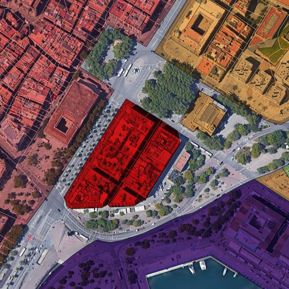
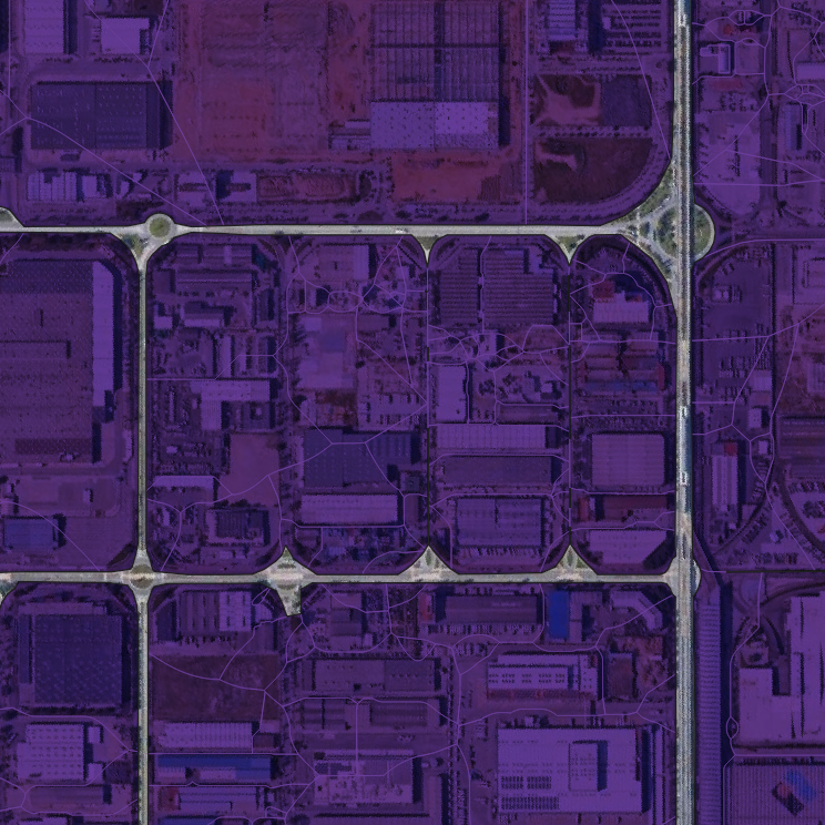
Figure 5.2: Islands produced by enclosed tessellation.
Arguably, there is some justification for having two-lane highways present a greater conceptual barrier than the wall between two buildings, but the absolute barrier effect found in the current implementation of ET is on balance too great. A possible alternative would be to keep the ‘empty’ ET cells generated, ignoring them when calculating morphometric characters based on information about buildings within the cells, but allowing their use at the contextual character stage. In this way the ‘empty’ ET cells would be assigned the average values of their neighbours, and not act as an absolute barrier when calculating contiguity-based spatial weights for contextual characters. Alternatively, an additional step could be added, using the ET cells as the input to a further Voronoi tessellation. In this way, any ‘empty’ spaces (those enclosures without buildings) would be divided according to their nearest (non-empty) ET cell and appended to these cells, creating a spatially exhaustive tessellation based on enclosures and in which every cell contains a building.
5.4 Creating spatial segmentations with different clustering algorithms
The results show that, while the segmentations generated are contingent on a number of different parameters, the Gaussian Mixture Model clustering algorithm used to produce the majority of segmentations is capable of building clusterings which accurately discern key urban tissues. The results of the segmentation produced using Agglomerative Clustering in place of GMM highlight the imperative role played by the choice of algorithm. Even when using identical input data, different algorithms (even when aiming to demarcate the same thing) can produce vastly different clusterings.